How we use discount rates to value business opportunities

How we use discount rates to value business opportunities

All of a sudden, the discounted cash flow (DCF) method is in the news. If you’re not a financial analyst, DCF probably doesn’t mean much to you. But recent comments by Australia’s Grattan Institute prompted me to explain how we go about valuing companies at Montgomery.

Readers of the blog will by now know that we at Montgomery generally use a DCF based framework to establish an intrinsic value of a company which is then compared to the value that the market is currently assigning to the company. An intrinsic value in excess of current market value suggests that the company is one we should consider investing in while a market value well above the intrinsic value indicates that we should stay away.

This post is an attempt to:

1. Show the importance of using an appropriate discount rate by showing how the importance of the terminal value differs with the discount rate used and
2. Provide a bit of comment on an article published recently by the Grattan Institute, which argues that Australia is taking the wrong approach to valuing big infrastructure.

Establishing the intrinsic value, in general and simplified terms, involves the following steps:

1. Establish a forecast of the cashflow a company can generate over an explicit forecast period taking into account the overall economic outlook, the specific industry drivers and the circumstances of the specific company like for example its existing assets, its competitive position, investment needs and its strategy etc.
2. Establish a terminal growth rate to be applied to the cashflow post the explicit forecast period (most businesses can be assumed to exists longer than we can forecast in detail unless they have assets of defined life when it is possible to do a DCF valuation without a terminal growth rate assumption). It is here important to be careful that you do not assume a growth rate that is well in excess of the long term economic growth rate as due to compounding effects, you can get large swings in value by small changes in assumptions which would indicate that the company/sector etc. would take a disproportionally large share of the total “economic pie” in the (long-term) future.
3. Establish a discount rate to discount the above-mentioned cash flows back to today and to establish the “terminal value” which is basically a multiple to be applied to the last explicit forecasted cashflow to account for the value of the cashflows that lies outside the explicit forecast period. This multiple can be determined in several different ways which I will not go into here but all off them includes the discount rate as a significant factor.

Mathematically, the intrinsic value calculation can then be described as:

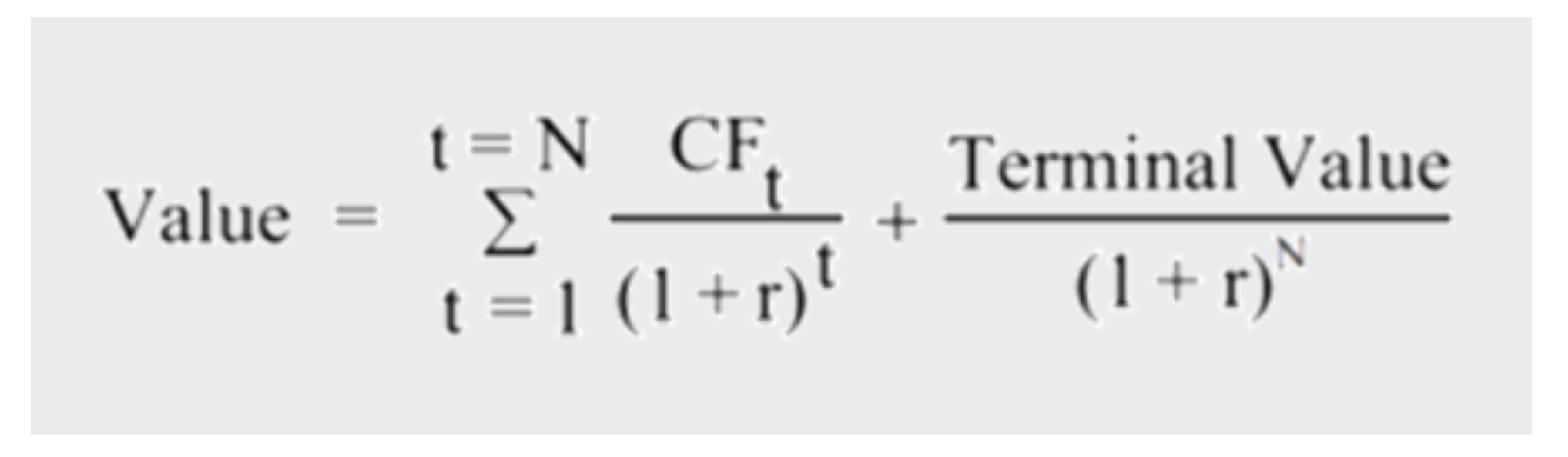
Where r = discount rate, CFt = Cash flow in period t and N = Number of explicit forecast periods.

As mentioned above, the Terminal Value can be calculated in many different ways but the most common way (but not always the most correct) is to use the perpetuity growth formula:

Where FCFt+1 = The cash flows in the period after the explicit forecast period ends, r = Discount rate and g = The assumed perpetuity growth rate.

As you can see, the discount rate influences both the Terminal Value directly and also the present value of the Terminal Value.

As an illustration of how large impact different discount rates can have on a DCF valuation, let us assume a company that is forecasted to have the following cashflows:

• First year cashflow is $100
• This cashflow is forecasted to grow by 5 per cent per year for the first 10 years
• Terminal growth rate is forecasted to be 2.5 per cent which can be said to be in-line with long term economic growth assumptions for the overall world economy.

The explicit cashflows for such a company would look like this chart which is basically 100 grown by 5 per cent for the first 10 years and then grown by 2.5 per cent for the 11^th year:

If we now look at the present values of the cashflows described in the chart above and calculate the Terminal Value according to the perpetual growth formula shown above for discount rates of 10 per cent, 8 per cent and 6 per cent, we get the following charts:

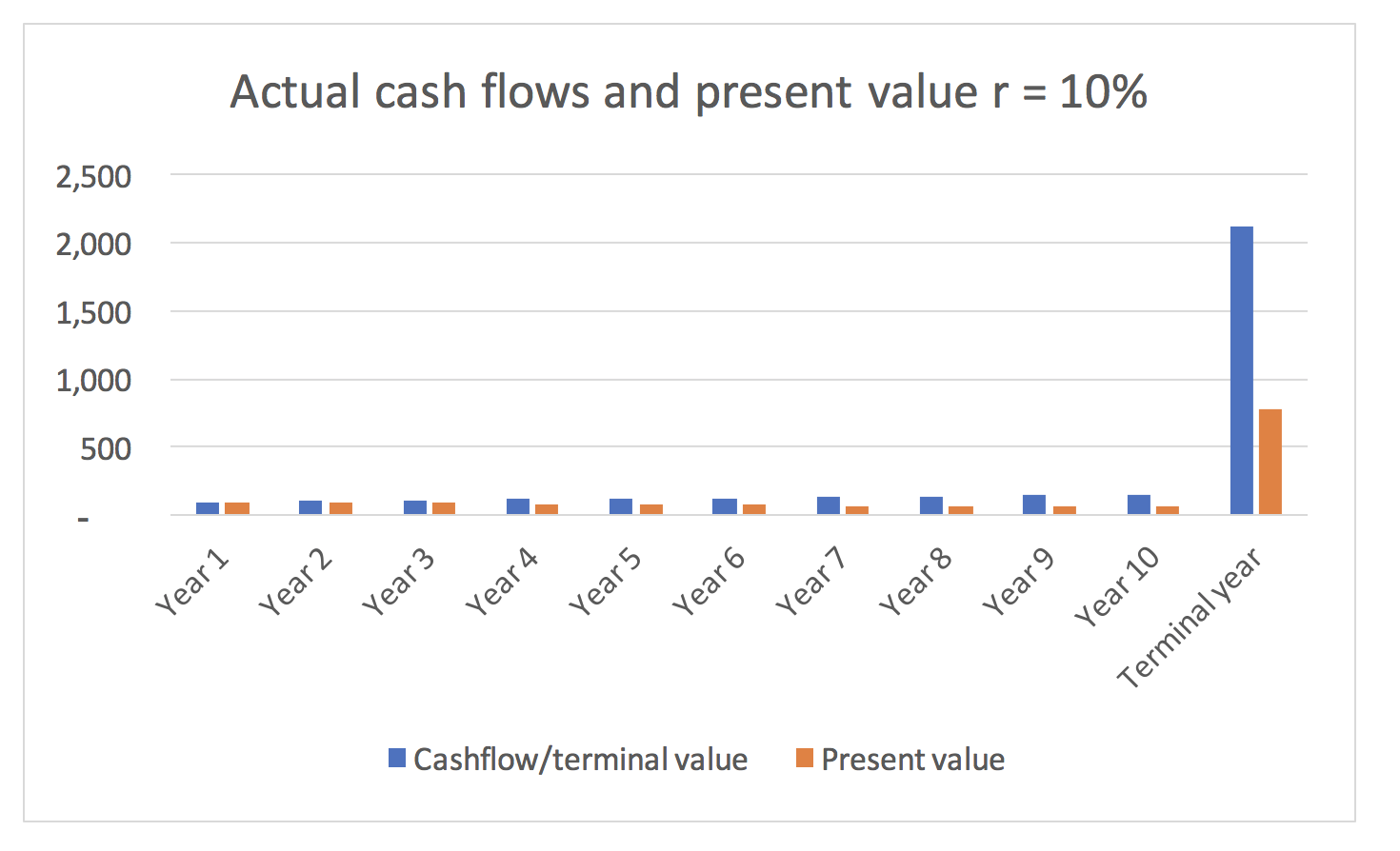
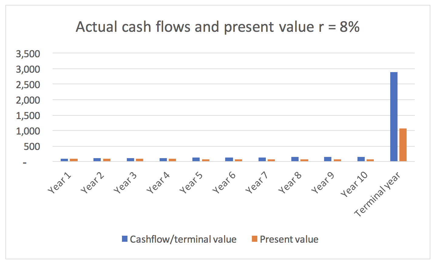
We can directly see that a significant portion of the total value for all discount rates lies in the terminal value term but what is interesting is how quickly the terminal value term increases in importance as the discount rate goes down. The table below shows how the portion of the total Present Value (PV) of that the Terminal Value (TV) accounts for the 3 different discount rates:

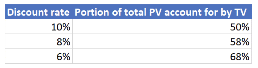
By going from 10 per cent discount rate where the TV accounts for 50 per cent of the total PV to 6 per cent where TV accounts for 68 per cent of total PV, we significantly increase the importance of the terminal value.

This does most likely not come as a surprise to anyone who has done much financial modelling before. We should though note that the difference between 10 per cent and 8 per cent discount rate is 8 per cent difference in the importance of the terminal value and the difference between 8 per cent and 6 per cent discount rate is 10 per cent difference in terminal value or in other words, the lower the absolute discount rate, the more difference does a change in discount rate make.

This is important for a couple of reasons:

1. We are currently in a historically very low interest rate environment and economic theory states that if the risk-free interest rates are low, the discount rates used to evaluate investments should also be low (type in CAPM in google if you are interested).
2. This means that higher importance will be placed on the terminal value.
3. It is hopefully obvious to any readers that the longer a forecast period is, the lower the accuracy of forecasts towards the end of the forecast period is.

This means that great care needs to be taken when choosing:

1. The length of the explicit forecast period and
2. The discount rate used

As especially using a low discount rate, especially in combination with a long explicitly forecast period leads to a very high reliance on the terminal value which by its very nature is very uncertain.

This leads to the second purpose of this post which is to express a bit of hesitation towards the article by Grattan Institute which argues that Australian government agencies should significantly lower the discount rate used to evaluate investments in transport infrastructure.

As a bit of background, Australian government agencies have since 1989 been using 7 per cent discount rates to evaluate the economic benefits of all transport investments. In the same period, real risk-free rates have fallen from around 7 per cent to around 0.8 per cent today. Grattan Institute are using this as an argument that Australian government agencies should instead 1. Vary interest rates over time according to what the risk-free rate is and 2. Vary the interest rate between projects according to their level of systematic risk (i.e. low correlation to overall economic activity) and move to use 3.5 per cent discount rate for projects with low systematic risk and 5 per cent for project with medium systematic risk.

The main argument for this is that the current one-size fits all discount rate penalises projects with longer dated benefits vs. projects with higher short-term benefits.

I have some sympathy for the notion that the discount rate should be somewhat different for projects with different risks; we at Montgomery are using the same approach in our analysis of companies as we apply a higher discount rate when we have less confidence in the accuracy of our forecasts and a lower discount rate when a company is easy to forecast with precision (think regulated utility vs. a growth IT company).

What I do have an issue with though, is the notion that interest rates should vary significantly over time. Interest rates go through cycles and can change significantly over time. Just because we are in a very low interest rate environment now does not mean that this situation will persist forever and decision taken at a specific point in the interest rate cycle can look very silly at another point in the interest rate cycle using a very different discount rate. I would argue that it is much better to use a long term average interest rate to ensure consistency over time.

I have also got an issue with using such absolute low numbers as 3.5 per cent as a discount rate. As can be seen from the example above, the lower the discount rate, the more importance is placed on the terminal value (or the far far out years if the explicit forecast period is very long) where the accuracy of the forecasts is by its very nature much less accurate. Basically, the lower the discount rate, the greater caution must be taken in not getting your assumptions used for forecasting wrong and a discount rate of 3.5 per cent does not give you much room for error in your forecasting!